COMPAS LnL Surrogate

This python package helps make an LnL surrogate for COMPAS SF-params given a set of BBH mergers. The surrogate is trained using active learning/bayesian optimisation techniques. This package acts as a bridge between the COMPAS LnL computer, surrogate modelling packages, and Bayesian optimisation packages.

Installation

pip install lnl_surrogate@git+https://github.com/COMPAS-Surrogate/lnl_surrogate.git

Example

from trieste.acquisition.function import PredictiveVariance, ExpectedImprovement


import numpy as np
from lnl_surrogate.surrogate import train
from scipy.stats import norm
from lnl_surrogate.surrogate.setup_optimizer import McZGrid
from lnl_computer.mock_data import generate_mock_data
from typing import Dict
import matplotlib.pyplot as plt
import os

np.random.seed(0)

MINX, MAXX = 0.005, 0.015
MIDX = (MINX + MAXX) / 2
NORM = norm(MIDX, 0.003)
OUTDIR = 'outdir'
os.makedirs(OUTDIR, exist_ok=True)

def mock_lnl(*args, **kwargs):
    sf_sample: Dict = kwargs.get('sf_sample')
    sf_sample = np.array(list(sf_sample.values()))
    return NORM.logpdf(sf_sample), 0

def plot_res(model, data, search_space):
    x = np.linspace(MINX, MAXX, 100).reshape(-1, 1)
    true_y = NORM.logpdf(x) * -1.0
    model_y, model_yunc = model.predict(x)
    x_obs = data.query_points
    y_obs = data.observations

    tf_to_np = lambda x: x.numpy().flatten() if hasattr(x, 'numpy') else x
    # make new fig
    plt.figure()
    plt.plot(x, true_y, label='True', color='black')
    plt.plot(x, model_y, label='Model', color="tab:orange")
    plt.scatter(x_obs, y_obs, label='Observed', color='black')
    yup, ydown = tf_to_np(model_y + model_yunc), tf_to_np(model_y - model_yunc)
    plt.fill_between(x.flatten(), yup.flatten(), ydown.flatten(), alpha=0.2 , color="tab:orange")
    plt.legend(loc='upper right')
    return plt.gcf()

McZGrid.lnl = mock_lnl
mock_data = generate_mock_data(OUTDIR)

acq_fns = [PredictiveVariance(), ExpectedImprovement()]
for acq_fn in acq_fns:
    res = train(
        model_type='gp',
        mcz_obs=mock_data.observations.mcz,
        compas_h5_filename=mock_data.compas_filename,
        acquisition_fns=[acq_fn],
        params=['aSF'],
        n_init=2,
        n_rounds=10,
        n_pts_per_round=1,
        outdir=f"{OUTDIR}/gp",
        truth=dict(
            aSF=MIDX,
            lnl=mock_lnl(sf_sample={'aSF': MIDX})[0]*-1.0
        ),
        model_plotter=plot_res,
        noise_level=1e-3
    )

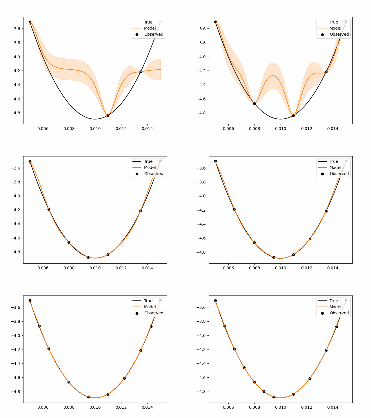
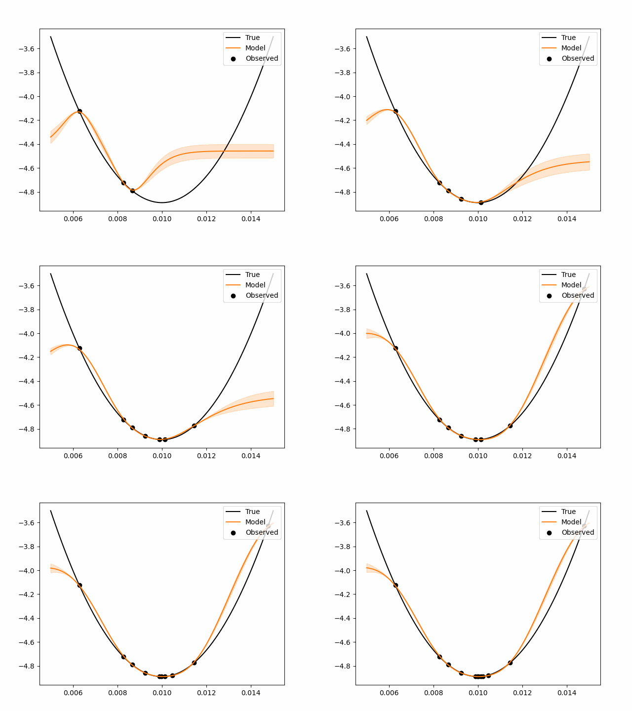
Exploratory Acquisition	Exploitative Acquisition