Bayesian Optimization for GPs#

GPs can provide a reconstruction of an unknown function from sparse measurements

Additionally, the GP posterior predictive mean, \(\mu\), and posterior predictive variance, \(\sigma\), can be used to derive an acquisition function, \(\alpha(\mu,\sigma)\). Acquisition functions are useful in selecting the next point to observe from the model in optimization problems (active learning).

We can select the next point using:

\[ x_{next}= \underset{x}{\arg\max}\frac{1}{N_{\rm{mcmc}}}∑_{i=1}^{N_{\rm{mcmc}}} \alpha(\mu^i,\sigma^i) \]

where

\(N_{\rm{mcmc}}\) is the total number of MCMC samples,
\(\mu^i\) is the i-th sample posterior predictive mean, and
\(\sigma^i\) is the i-th sample posterior predictive variance.

There are several acquisition functions that can be used.

Acquisition functions#

An acquisition function is a function that maps the posterior predictive mean and variance to a scalar value. The scalar value is used to select the next point to observe from the model.

In general, we will write the acquisition function as \(\alpha(\mu,\sigma)\), where \(\mu\) is the posterior predictive mean and \(\sigma\) is the posterior predictive variance.

Penalizing Recent Observations#

We can add in a penalty factor based on the recently observed points to avoid sampling the same region of the function space repeatedly.

This can be tacked on to some acquisition function as follows:

\[ \alpha(\mu,\sigma) - \lambda\ \gamma(x, \vec{X_{\rm r}}) \]

where \(\lambda\) is some penalty factor and \(\gamma(x, \vec{X_{\rm r}})\) is the penalty for point \(x\) based on their distance to the recently visited points \(\vec{X_{\rm r}}\).

The Upper Confidence Bound (UCB)#

The upper confidence bound (UCB) acquisition function is defined as

\[ \alpha_{\rm{UCB}}^i(\mu^i, \sigma^i)= \mu^i\pm\sqrt{\beta\ \sigma^i}\qquad \]

The coefficient \(\beta\) determines an exploitation-exploration trade-off.

Note

The primary goal of UCB is to find a global minima/maxima rather than to reconstruct the entire function accurately.

This is an animation of using UCB to help choose the next points for a GP

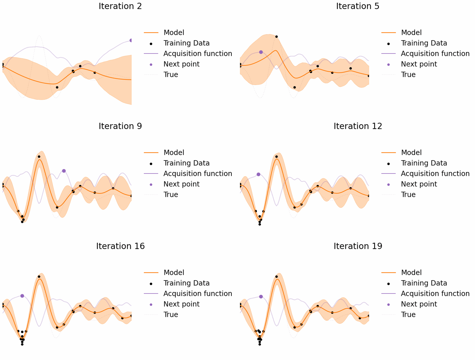
This is the same animation but with adding in a penalty factor:

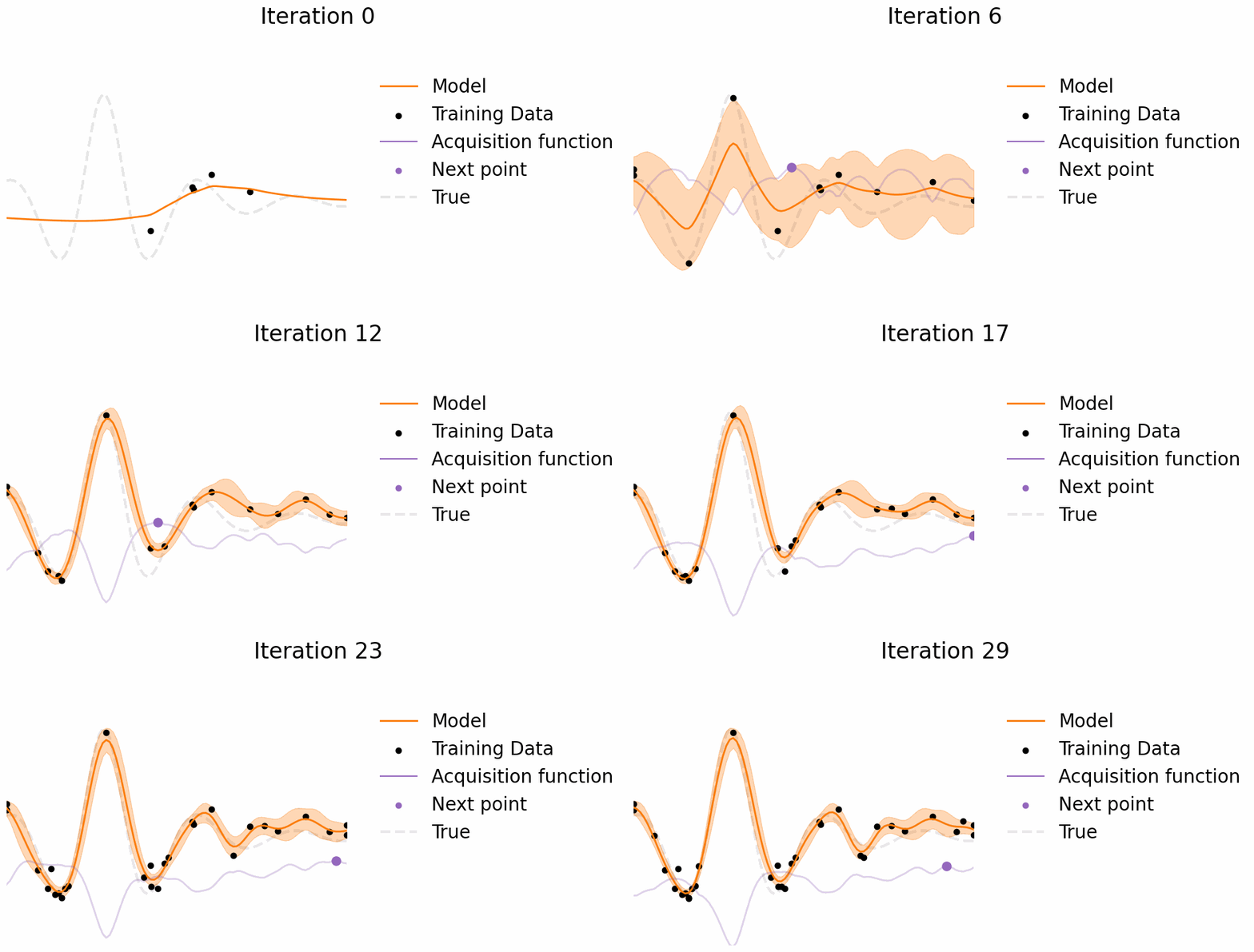
A drawback of this method is that it requires an update of the GP model after each new observation. This can be computationally expensive.

Here are some more examples:


D1
D2
D3

Batched UCB (qUCB)#

In MCMC-based GP, we obtain a separate multivariate normal posterior for each set of sampled kernel hyperparameters. Hence, we can create a separate UCB acquisition function for each posterior, and then acquire a batch of new points.

The following are two animations made with different random seeds (no penalty factor).

Thompson Sampling#

Thompson Sampling uses the following logic:

Fit the GP to the observations we have
Draw one GP sample (a function) from the posterior
Greedily choose the next point x with respect to the sample

See wikipeda

As this method is probabilistic, it does not need to be updated after each new observation.

Here are some examples:


D1
D2
D3

Uncertainty-based exploration (UE)#

This acquisition function aims at reducing the uncertainty of the GP model. It is defined as

\[ \alpha_{\rm{UE}}^i(\sigma^i)= \sigma^i \]

and helps to explore the function space in regions of high uncertainty.


D1
D2
D3

Expected Improvement (EI)#

This also focuses on the maximisation/minimisation of the GP’s posterior predictive mean. It looks for the best value of \(\mu\) so far and then looks for the next point that has a higher probability of being better than the best value so far.

\[ \alpha_{\rm{EI}}^i(\mu^i, \sigma^i)= \sigma^i\ (u^i \mathcal{N}_{\rm CDF}(u^i) \mathcal{N}_{\rm PDF}(u^i)\ , \]

where \(u^i = \frac{\mu^i - \mu_{\rm{best}}}{\sigma^i}\) and \(\mu_{\rm{best}}\) is the best value of \(\mu\) so far.


D1
D2
D3

Table of all anim#

	D1	D2	D3
EI
TH
UCB
UE
MSE